0

I want to create a function for a curve which is similar to a sigmoid curve but the center part is linear. That curve must pass through 2 points (-1.5,20) and (1.5,80). The range for y value is [0,100]. I have create two functions which are shown in the figure below.

http://i827.photobucket.com/albums/zz197/koifish1987/curve_zpsaju4fxhn.jpg

sigmoid curve: $y = \frac{{100}}{{1 + {e^{ - \frac{{\ln 4}}{{1.5}}x}}}}$

linear line: $y=20x+50$

I want to make the sigmoid curve (black) closer to the linear line (red). How can I change the sigmoid function to achieve that? Or is there any function which yields the similar curve shape and more linear in the center?

opmfan
  • 5

1 Answers1

0

You can add terms in the exponent to cancel higher derivatives at the origin. They need to be antisymmetric, and they shouldn't mess up the behaviour at infinity. Powers of $\sin x$ satisfy those requirements. To cancel the third derivative:

$$ \frac1{1+\exp\left(-x-\frac1{12}\sin^3x\right)}=\frac12+\frac x4+O\left(x^5\right)\;. $$

To cancel the fifth derivative:

$$ \frac1{1+\exp\left(-x-\frac1{12}\sin^3x-\frac{13}{240}\sin^5x\right)}=\frac12+\frac x4+O\left(x^7\right)\;. $$

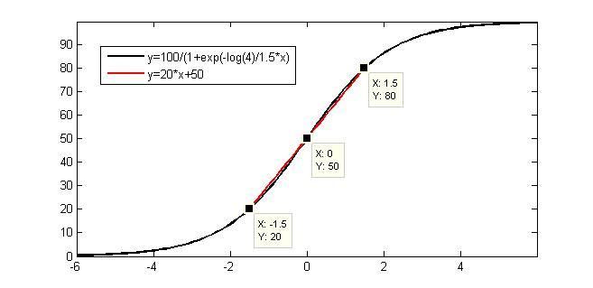
And so on. Here's a plot of the second version.

This comes at a price – forcing the function into an "unnatural" linearity at the origin while keeping it analytic causes slight oscillations elsewhere. Of course, if you don't care about analyticity, you should just splice a linear function into a sigmoid.

P.S.: I was assuming that you want to keep the asymptotic behaviour roughly unchanged. If you don't care about that, you can do it more simply:

$$ \frac1{1+\exp\left(-x-\frac1{12}x^3\right)}=\frac12+\frac x4+O\left(x^5\right)\;. $$

The plot looks a lot like what you wanted, but it converges to the limit more rapidly than a sigmoid.

The next step in that direction would be

$$ \frac1{1+\exp\left(-x-\frac{x^3}{12}-\frac{x^5}{80}\right)}=\frac12+\frac x4+O\left(x^7\right)\;. $$

And, since you wanted to have an $x^7$ term for rapid convergence, here's the next step, too:

$$ \frac1{1+\exp\left(-x-\frac{x^3}{12}-\frac{x^5}{80}-\frac{x^7}{448}\right)}=\frac12+\frac x4+O\left(x^9\right)\;. $$

At this stage, the plot looks very linear indeed – if you go any further, you might as well use a linear function with cut-offs at both ends instead :-)

joriki
  • 238,052
  • Hi joriki, Thank you very much for your answer. I found that the third function you gave me is very close to what I want.

    Actually, I want to model a response curve of image sensor to brightness of the scene. This curve is quite similar to the one I plotted using my previous sigmoid function.

    This curve passes two point (-1.5,20) and (1.5,80) because I assume that for the pixel value from 20 to 80, an increment of brightness would increase the pixel value to 20.

    – opmfan Aug 06 '15 at 16:09
  • My previous curve is not correct in 3 points: (1) the center is not linear (2) the varying of brightness is not that long, It should be -4 to 4, not -6 to 6. So the curve should converge to the limit more rapidly and I could get rid the part beyond [-4,4].. (3) the slope of the curve before the 20 and after 80 should be a little bit higher. (so the curve should converge more rapidly) – opmfan Aug 06 '15 at 16:29
  • @JamesDo: You're welcome. Since you said that the third function was more useful, I also added the corresponding function with an $x^5$ term to the answer. On your second comment: great coincidence, then, that problems (2) and (3) happened to be addressed by the solution to problem (1) :-) – joriki Aug 06 '15 at 16:29
  • From your third function I found that this function is close to what I need y=1/(1+exp(-ln(4)/1.5*x-x^7/7000)). For the linear part, I use the linear function y=20x+50. The plot of the new curve is shown here

    http://i827.photobucket.com/albums/zz197/koifish1987/curve1_zpsmnaozc5d.jpg

    The curve does not meet the linear section at two point (-1.5,20) and (1.5,80). But this is enough for me ^.^

    – opmfan Aug 06 '15 at 16:31
  • @JamesDo: I see. (Note that there's an $x$ missing in the equation in the image.) – joriki Aug 06 '15 at 16:36
  • You're right. x is missing in my figure. I choose the coefficient of -ln4/1.5 for x since I want the curve almost pass two points (-1.5,20) and (1.5,80). The higher order of the additional term makes the curve converge more rapidly (so x^7 instead of x^3). And I found that I need to high denominator for x^7 so that the curve get closer to those two points. Also a high denominator seems to eliminate the wavy things at two ends of the curve. Do you have any better idea? – opmfan Aug 06 '15 at 16:55
  • @JamesDo: If you wanted the $x^7$ for fast convergence, I'd suggest to include all the terms up to $x^7$ to make the curve as linear as possible. I've added the corresponding function at the end of the answer. Note that it has a much larger $x^7$ term, so it's both "more linear" and converges faster. – joriki Aug 06 '15 at 17:03
  • As you suggest in the answer, I think I just need to splice a linear function into a sigmoid. Your final function make the center part is very close to linear. But the center part does not match the linear section (the red line in the image below).

    http://i827.photobucket.com/albums/zz197/koifish1987/curve2_zpswesbdkhn.jpg

    I wonder if your function can be change somehow to match the linear section, especially at the two end of the linear section (red line).

    – opmfan Aug 06 '15 at 17:27