Yes, by the structure of the equation it is the only stationary point.
If $b+x^3-Tx>\sqrtϵ$, then $\dot x\sim -\frac1{\sqrtϵ}$ moves the flow fast to the left stopping at the falling branch of $b=Tx-x^3$. Similarly for $b+x^3-Tx<-\sqrtϵ$. For a point close (meaning with distance $O(ϵ)$) to the falling segments of the graph of the cubic, and assuming that $x_0$ is between the locations of the maxima and minima of the cubic, the first equation forces the flow towards the cubic while the second one moves $b$ towards the extremum next to the current position, downwards for negative $x$ and upwards for positive $x$. Thus the flow of the system creeps down the negative falling branch until it reaches the minimum where it leaves the cubic and is blown to the positive falling branch. There it creeps upwards until it reaches the maximum, is blown to the left and so on.
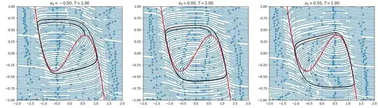
To find a contour where the vector field points uniformly inwards seems complicated.
The following is incomplete. While the theory of Lienard systems is more general, the described Lyapunov functions work only under the assumption $c(u)\ge 0$.
Consider the second order form $ϵ\ddot x+(3x^2-T)\dot x+(x-x_0)=0$ and compare to the form of a Lienard equation
$$
u''+c(u)u'+g(u)
$$
as in Stability in a Liénard system.
This is achieved by setting $u=x-x_0$, $g(u)=\frac uϵ$, $c(u)=\frac1ϵ(3(x_0+u)^2-T)$. Then the Lyapunov function proposed in the answer is, using $p=\dot u$
$$
V(u,p)=\frac12\left(p+C(u)\right)^2+\frac12p^2+2G(u),\\~\\C'=c,~G'=g,~C(0)=0=G(0)
$$
with derivative along the solutions of
\begin{align}
\dot V&=-(p+C(u))\,g(u)-p\,(c(u)p+g(u))+2g(u)\,p
\\
&=-C(u)\,g(u)-p^2\,c(u)
\\
&=-\frac1{ϵ^2}(u^2+3ux_0+3x_0^2-T)u^2-\frac1ϵ(3(x_0+u)^2-T)p^2
\end{align}
Assuming $3x_0^2<T$, this is positive around $(u,p)=(0,0)$ and negative for $(u+\frac32x_0)^2>T$ or $|p|$ large enough. Thus you can identify a region with a hole around $(0,0)$ where the system has no stationary points and the vector field flows inwards on the boundary. Now apply Poincaré-Bendixon.
How to get this (Lyapunov?) function, start with the usual, multiply with $u'$ and integrate, you get that $$\frac12u'^2+G(u)=-\int c(u)u'^2\,dt.$$ Use partial integration on the right side, $$\int c(u)u'^2\,dt=C(u)u'-\int C(u)u''=C(u)u'+\int C(u)(c(u)u'+g(u))\,dt=C(u)u'+\frac12 C(u)^2+\int C(u)g(u)\,dt.$$ Now insert and combine to complete squares
$$
\frac12(u'+C(u))^2+G(u)=-\int C(u)g(u)\,dt
$$
The first right side has an integrand that is a multiple of $u'^2$, the second integrand is a multiple of $u^2$. Use the sum of both to get both coordinates involved. Then use handwaving to make the segment where $c(u)<0$ negligible?
Appendix: Code for the plots
import numpy as np
from matplotlib import pyplot as plt
from scipy.integrate import odeint

eps=0.1; T=1.0;
def odesys(y): x,b = y; return [ -(b+x**3-T*x)/eps, x-x0 ];

x_lim = [-2,2]; y_lim = [-1,1]
X, B = np.meshgrid(np.arange(x_lim[0], x_lim[1]+0.01, 0.1), np.arange(y_lim[0], y_lim[1]+0.01, 0.1))

x_cub = np.linspace(x_lim[0], x_lim[1], 501);
b_cub = T*x_cub-x_cub**3;
t_sol = np.linspace(0, 20, 2501);

for k in range(3):
     x0 = [ -0.5, 0, 0.5][k]*T**0.5;
     a= (T/3.0)**0.5 # extrema at -a, +a; -a < x0 < a
     plt.subplot(1,3,k+1);
     plt.ylim(y_lim);
     plt.plot(x_cub, b_cub,'r', lw=2);
     dotX, dotB = odesys([X,B]);
     plt.streamplot(X, B, dotX, dotB, density=2.5);
     y_sol = odeint(lambda y,t: odesys(y), [(T/3)**0.5, 2*(T/3)*(T/3)**0.5], t_sol, atol=1e-9, rtol=1e-10);
     x_sol, b_sol = y_sol.T; plt.plot(x_sol, b_sol, 'k', lw=1.5);
     plt.grid(); plt.title('$\epsilon=%.2g$, $x_0=%.2f$, $T=%.2f$'%(eps,x0,T));
plt.show();


