Here is an elementary example of the use of a density estimator in R.
First we generate a thousand observations from the gamma distribution $\mathsf{Gamma}(\mathsf{shape}=\alpha=2, \mathsf{rate} = \lambda = 1/3)$
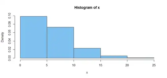
and plot their histogram in such a way that the 'modal bin' includes the smallest values.
set.seed(327)
x = rgamma(1000, 2, 1/3)
hist(x, prob=T, br=7, col="skyblue2")
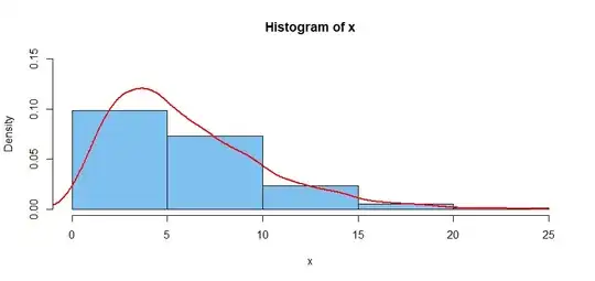
Then we find the default density estimator in R. It consists of 512 points. Plotting them imitates a smooth curve.
den.est = density(x)
hist(x, prob=T, br=7, ylim=c(0,.15),col="skyblue2")
lines(den.est, type="l", lwd=2, col="red")
Here is a summary of the $(x,y)$ points of the density estimator.
We can use these points to find where the estimated density curve
is at its highest points. Thus, we can locate the 'mode' of the data, as defined by the density estimator. For our simulated data its about $3.65.$ (We take the 'mean' of x's with highest y-value because there may
be ties.)
den.est

Call:
        density.default(x = x)

Data: x (1000 obs.);    Bandwidth 'bw' = 0.8625

       x                y
 Min.   :-2.480   Min.   :6.260e-06
 1st Qu.: 4.383   1st Qu.:2.507e-03
 Median :11.247   Median :1.828e-02
 Mean   :11.247   Mean   :3.639e-02
 3rd Qu.:18.110   3rd Qu.:6.596e-02
 Max.   :24.974   Max.   :1.203e-01

mean(den.est$x[den.est$y == max(den.est$y)])
[1] 3.644313
Usually the point of finding the mode of a histogram is to estimate the mode of the population distribution. We did pretty well in this example: The gamma distribution $\mathsf{Gamma}(\alpha=2,\lambda=1/3),$ from which we simulated the data
has its mode at $(\alpha-1)/\lambda = 1/(1/3) = 3.$
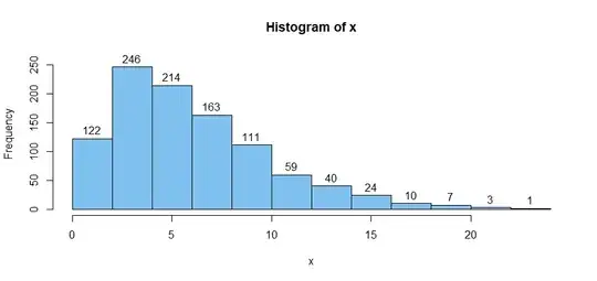
Note: By way of full disclosure: (1) With as many as $n = 1000$ observations, we might have used more bins in our
original histogram so that the traditional formula could be used. Here is a frequency histogram of the data with more bins. (I will leave it to you to see what value the traditional method gives.)
hist(x, ylim=c(0,260), labels=T, col="skyblue2")
(2) Also, if the population distribution has its mode at
one end of its support, a modification of the default kernel density estimator in R may be required for a good
estimate of the mode. (An exponential distribution, with its
'mode' at $0,$ would be an example.)


