This sounds like a Beta-Binoimial purchase rate model would be useful. The link has a lot of details on this, but I'll give the salient highlights:
- We are assuming that when a product $i$ is introduced, we are uncertain as to its actual bought rate $BR_i$. We model this uncertainty with a beta distribution on [0,1]. For example, the uniform distribution on [0,1] is a member of the beta family of distributions.
- As the data roll in, you will get updates on the number of views, $n_i$ and the number of buys $x_i$ for each product $i$.
- Use this data to derive a "shrinkage estimate" of the bought rate. The details are well spelled out in the link and are too long to reproduce here. However, I've snipped the key equations from the wiki article and placed them below:
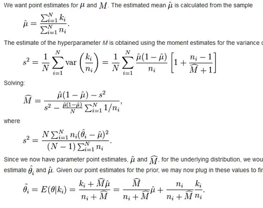
- These estimates will prevent over-weigting of "chance" occurrances such as 1 look - 1 buy, which are spurious and over-estimate the actual BR (and vice versa for 1 look, no buy).
Now, what about deciding which products to show? Since your product mix changes a lot, I would suggest considering a semi-randomized method of displaying products.
- Rank all your products by estimated BR (using all current data and the beta-binomial model)
- Add up the estimated BR for all products, and divide each BR by this sum. This will create a empirical distribution based on the current BR estimates.
- When a user starts viewing pages, you will want to populate the pages by selecting, without replacement, from the distribution you created in (2).
- Periodically re-evaluate your estimates based on current data.
This will both prevent over/under estiamtes based on only a few results and will give new products a chance to be seen and further evaluated.
Anyway, just suggestions. Hope it helps.
Specific example:
Lets say you have N products on your website. The number of times a product $i$ has been viewed is $v_i$, and the number of times bought is $b_i$. Therefore the naive estimate of the bought rate is $\frac{b_i}{v_i}$. However, this will lead to erratic results for new products. Instead, we will adjust this estimate using the beta-binomial model.
- Calculate the "grand mean" bought rate of all your products: $\hat \mu = \frac{\sum b_i}{\sum v_i}$. What we are doing here is creating an "anchor" for the observed bought rates. The remaining calculations will determine how far away from this mean rate we should allow each product's BR estimate to get.
- Calculate "Grand variance":
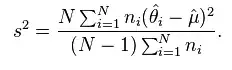
Where $\hat \theta_i = \frac{b_i}{v_i}$
Almost done....
- We are going to use our estimates of $\hat \mu$ and $s^2$ to calculate $\widehat M$, which determines how much weight we will give to $\hat \theta_i$ vs $\hat \mu$ in our estimate of the bought rate.
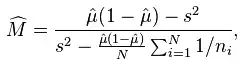
- Once you have $\widehat M$, you have everything you need to estimate your bought rates, given the data. This will result in a "shrinkage factor" for product $i$:
$\widehat B_i = \frac{\widehat M}{\widehat M + v_i}$
Putting all this together, our revised estimate of the bought rate for product $i$ is:
$BR_i = \widehat B_i \hat \mu + (1-\widehat B_i)\frac{b_i}{v_i}$
