Here is a complete remodeling of my previous answer.
Take a look at Fig. 1.
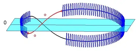
Fig. 1.
This figure represents the central part of the rubber band constituted of 2 circle arcs (in blue) and 2 cubic Bezier curves connecting them (in red and black resp.), preserving not only continuity but also the differentiability at the connecting points between circular arcs and Bezier curves. The left cylinder has been tilted from an initial vertical position by an angle $a$
($a=\pi/6$ here) around $Ox$ axis represented here splitting the horizontal plane into two parts. The right cylinder has been tilted by an opposite angle $-a$.
The four points that define one of the Bezier curve (the red one) are pictured as small circles. Two of them are clearly obtained as endpoints of the circular arcs, the other two are obtained by approximating speed vectors at the said endpoints.
You will find at the end the Matlab program that has generated Fig. 1.
Fig. 2 is a compulsory aid in order to understand the situation before the cylinders are tilted and the numerous implementation details :
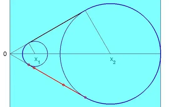
Fig. 2.
Remark : the conventions taken are WLOG (Without Loss Of Generality) : in particular, Ox axis has been selected as directed by the shortest line segment between the cylinders. And through this axis, there always exists a plane such that the axes of the two cylinders make angles $\pm a$ with this plane.
 function rubberband;
 clear all,close all;hold on;axis equal;
 LW='linewidth';
 x1=5;x2=12;% abscissas of centers
 a=pi/6;% angle under which the circles are seen from 0
 sa=sin(a);r1=x1*sa;r2=x2*sa;
 view([4,6]);
 co=50;
 b=pi/6;%tilt angle of cylinders
 h=1;% cylinders half height
 R1=[1,0,0;
      0,cos(b),-sin(b);
      0,sin(b),cos(b)];% rotation matrix around Ox
 R2=inv(R1);
 % The horizontal plane:
 D=9;fill3(D*[-1,1,1,-1,-1]+10,D*[-1,-1,1,1,-1],...
 zeros(1,5),'c','edgecolor','b','facealpha',0.5);
 plot3([0,2*D],[0,0],[0,0]);% x axis
 text(0,0,0.3,'0');% origin O
 t1=(pi/2+a):0.01:(3*pi/2-a);
 t2=fliplr((-pi/2-a):0.01:(pi/2+a));
 L1=length(t1);
 L2=length(t2);
 arc1=R1*[x1+r1*cos(t1);r1*sin(t1);zeros(1,L1)];
 arc1=R1*arc1;
 B=arc1(:,L1);plot3(B(1),B(2),B(3),'or');
 Bb=arc1(:,L1-1);
 VB=B+co*(B-Bb);plot3(VB(1),VB(2),VB(3),'or')
 rc2=[x2+r2*cos(t2);r2*sin(t2);zeros(1,L2)];
 arc2=R2*arc2;
 E=arc2(:,L2);plot3(E(1),E(2),E(3),'or');
 Eb=arc2(:,L2-1);
 VE=E+co*(E-Eb);plot3(VE(1),VE(2),VE(3),'or')
 % the two circle arcs:
 plot3(arc1(1,:),arc1(2,:),arc1(3,:),'b',LW,2)
 plot3(arc2(1,:),arc2(2,:),arc2(3,:),'b',LW,2)
 % the two cubic Bezier curves (see function below):
 bez(B,E,VB,VE,'r',0);
 bez(B,E,VB,VE,'k',1);
 % Cylinders plot:
 Cyu=[x1+r1*cos(t1);r1*sin(t1);h*ones(1,L1)];%up
 Cyb=[x1+r1*cos(t1);r1*sin(t1);-h*ones(1,L1)];%bottom
 Cy=R1*[Cyu,Cyb];
 for q=1:10:L1;
     plot3(Cy(1,[q,q+L1]),Cy(2,[q,q+L1]),Cy(3,[q,q+L1]),LW,2);
 end;
 Cyu=[x2+r2*cos(t2);r2*sin(t2);h*ones(1,L2)];%up
 Cyb=[x2+r2*cos(t2);r2*sin(t2);-h*ones(1,L2)];%bottom
 Cy=R2*[Cyu,Cyb];
 for q=1:5:L2;
     plot3(Cy(1,[q,q+L2]),Cy(2,[q,q+L2]),Cy(3,[q,q+L2]),LW,2);
 end;
 %
 function bez(B,E,VB,VE,col,sym);
 t=0:0.01:1;s=1-t;
 P=B*(s.^3)+3*VB*((s.^2).*t)+3*VE*((t.^2).*s)+E*(t.^3);
 if sym
     P=diag([1,-1,-1])*P;% symmetry wrt Ox axis
 end;
 plot3(P(1,:),P(2,:),P(3,:),'linewidth',2,'color',col)


